A Meandering Journey Towards the Source of Zeros
A few years ago, we started running triplicate technical PCR replicates for all of our eDNA metabarcoding samples. We had seen a lot of variation in some preliminary eDNA deployments and we thought it was worth capturing that variation (Kelly et al. 2018; Gallego et al. 2020; Gold 2020). The variation was real and often incredibly substantial, explaining upwards of a third of the data. It was clear that this variation was important, but we had no good explanation for why we were seeing it. We were doing everything in the lab identically for each technical PCR replicate. So, what on earth could be causing us this much variability?
For a long time, we had no good answers. We were surrounded by variation in our observed sequence reads and could not make out any obvious patterns. A lot of our data was from eDNA samples taken from the environment. Maybe they were just inherently noisy, noisier than microbiome datasets. Maybe we just had to accept the apparent chaos of eDNA metabarcoding.
But we didn’t take “it’s so random” for an answer.
So instead, we looked for a mechanistic driver. Something to explain what was going on with our data… So, working from home during the pandemic, I started making 2,000+ ggplot figures. Slicing and dicing the analyses every which way I could think of.
There were a lot of bad plots…
a lot of dead ends…
a lot of resigned slack messages in the “tears and whiskey” channel in the Kelly lab… A solid 6 months of clocking in and out and getting no closer to an answer…
But then we started looking specifically at our most unique dataset – a side-by-side comparison of metabarcoding vs. microscopy from CalCOFI samples. We had one jar of ethanol where we pipetted off the preservative and filtered it for “eDNA” and a separate paired jar taken from the other side of the bongo net tow preserved in formalin and expertly identified by the incredible CalCOFI taxonomists. Now we had a data set where we knew which species and how many to expect in every jar. We had a chance to understand what was driving this huge observed and unexplained variation in our metabarcoding data.
To make the case and point, here’s an example of what our technical replicates looked like for Snubnose blacksmelt (Bathylagoides wesethi) in one sample:
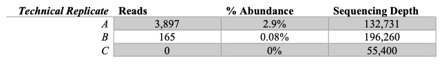
The variability in observed sequence reads and percent abundance is huge here and the zero is just totally unexpected given that there were over 3K reads in a sister technical replicate.
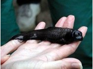
The source of zeros. Cute, but cursed.
However, now that we had an independent estimate of abundance to compare these results to, we could start to explore our data a little better:
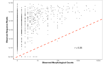
Figure 1. Observed Sequence Reads vs. Morphological Counts from CalCOFI dataset
The first thing we realized here is that yes, this is in fact super noisy data. There is a positive correlation for sure, but it’s also a pretty bad fit (even after drinking 6 beers). You could log transform the axes or even put it to the fourth root, but that doesn’t help us explain what is going on here. We wanted answers to why our data is the way it is, not a band-aid to an R2 value (p value hunting is strongly frowned upon).
However, 2 things immediately jump out from Figure 1 that gave us a clue for what to do next. First, there are actually quite a few non-detections lying across the x-axis. Places where our CalCOFI taxonomists saw a baby fish and we, using our fancy DNA metabarcoding, completely whiffed. What gives? Second, the variability in metabarcoding is way higher when there are fewer baby fish and the variability appears to decrease as there are more and more fish in a jar. So there were some important patterns in the data worth exploring.
From here we really wanted to understand what was driving this variability in sequence reads for rare targets. And in particular, something strange seemed to be going on with zeros, or non-detections. We only whiff with metabarcoding when there are less than 10 larvae. If there’s over 3,000 Anchovy in a jar or even 11 Anchovy in a jar, metabarcoding never misses. But rare fish are not always detected…
Now at the same time as this, we had been working on another rad, incredible, very cool paper showing how amplification efficiencies and underlying DNA concentrations can explain the number of observed reads, or the biological signal.
[For those of you too lazy to click the links and actually read the papers: we argue that the PCR process is a big driver of our observed reads: Amplicons = DNA Concentration (Amplification Efficiency) NPCR. Where amplification efficiency is how well a given molecule amplifies during PCR. A value of 1 meaning it doubles every time and a value of zero meaning your assay doesn’t work for that species at all. NPCR in this equation is how many PCR cycles.]
However, our quantitative metabarcoding framework does not explain the observed noise in our metabarcoding dataset. In particular, it does not immediately explain why there were so many zeros in our data. So, we set out to see if the same two variables that explain the biological signal (DNA concentration and amplification efficiency) of metabarcoding data also explained our noise.
And what we found next honestly stunned us.
First, we decided to make a bunch of mock communities in the lab to test our hypotheses. Basically, we made a bunch of fake fish communities where we knew how much DNA was loaded into each sample. This let us know 1) the starting DNA concentration and 2) the amplification efficiencies calculated from our trusty model. And out of a good fortune of sheer laziness in not wanting to standardize all the mock communities to the same copies per µL per species, we ended up with the perfect data set. So with that data in hand, we could see if the number of non-detections, zeros across technical replicates, was a function of 1) underlying DNA concentrations and 2) amplification efficiencies.
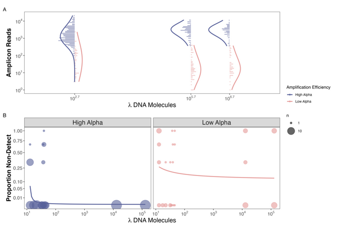
Figure 1. Observed Reads and Non-detections are a function of Amplification Efficiency and Input DNA Concentration in the Mock Community example
And low and behold we found that species that non-detections only occurred in species with high amplification efficiencies when there were very few copies of DNA (<30 copies/µL) in a mock community. At the same time, we saw non-detections at insanely high concentrations of DNA
for species with low amplification efficiencies (Figure 2b). On top of that we confirmed the results of our previous work showing that if you amplify well, you generate more reads per input DNA molecule (Figure 2a).
So of course, we realized we could make the exact same figure from the CalCOFI dataset now that we had known amplification efficiencies for 17 species from the mock community data. And boom: we got nearly identical results:
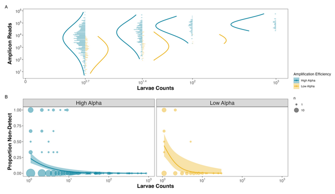
Figure 2. Observed Reads and Non-detections are a function of Amplification Efficiency and Larval Abundances in the CalCOFI example
At this point, we felt like we were really on to something, and I was ready to call it done.
Of course, though we had observations and a suggested underlying mechanism, we didn’t have any math. And that was not going to slide for the eDNA collaborative, particularly Ryan and Ole. We needed math, not just because they love math maybe more than fish, but to help us understand the patterns of the underlying mechanisms and provide us with a direct set of hypotheses to test. Sure, this might have been exactly backward to how one is supposed to make discoveries, but c’est le science. We did the math at the end.
I won’t dive into the details of the math in a blog post, so instead I just offer you the wonderful experience of taking a nice vacation in Ole and Ryan’s brains for 1,000 words while reading the methods section. The equations outline in detail our main findings: which are that noise is thus a function of 1) a stochastic sub-sampling process and 2) a PCR process with both a deterministic and stochastic component. Basically, we are saying zeros occur because 1) when you pipette rare things there is a higher chance you whiff and miss your target DNA molecule, 2) species with low amplification efficiencies are getting outcompeted by species that amplify better, and 3) not all the molecules made in PCR end up on the sequencer.
Running simulations, we find nearly identical patterns as we observed in our empirical datasets (Figure 3).
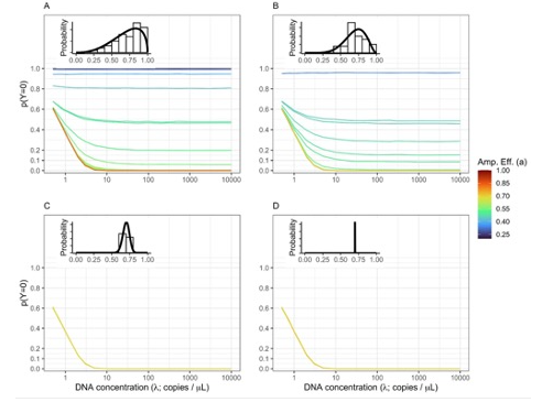
Figure 3. Non-detections Driven By Both DNA Concentration and Amplification Efficiency.
And so what we see that noise, just like signal, in metabarcoding datasets is a function of 1) underlying DNA concentrations and 2) amplification efficiencies. So why do we get zeros across technical replicates? Because your target is rare or your target amplifies relatively poorly with your given metabarcoding assay.
Now what do we do with this… read the next blog 🙂
Zack’s (misguided) road map to solving quantitative metabarcoding
TL;DR any of our mentioned pre-prints or previous blog post: we believe that observed patterns of sequence read abundance and non-detections from metabarcoding data are a function of 1) underlying DNA concentrations and 2) amplification efficiency and therefore are also a function of 3) what species are in the community, and 4) the proportional abundance of species in the community.
So now that we think we know this, how do we actually go about getting accurate quantitative metabarcoding estimates? I argue that you need to do 5 things to get quantitative metabarcoding estimates, some of which are simple, some are downright annoying, and some have never been done before in all of human history.
Do you accept this quest?
1. Independent estimates of underlying DNA concentrations.
The first thing that should be obvious at this point is that our PCR equation [Amplicons = DNA Concentration (Amplification Efficiency) NPCR] has 1 variable and 2 parameters. So just getting amplicon data from metabarcoding will not let you solve for the underlying DNA concentrations which is what we actually care about. And as I highlighted in the previous blog post, non-detections are also a function of underlying DNA concentration. And because metabarcoding is conditional, metabarcoding data at best can give your relative abundances. So for all of these reasons, it becomes very clear that we need to know the underlying DNA concentrations and amplification efficiencies for our species in addition to observed sequence reads from metabarcoding data.
At this point, you might be saying: “Dude, the whole point of me using metabarcoding in the first place is to know the underlying DNA concentrations of all the different species. You are telling me we need the answer to get the answer?” And I would reply, “It’s certainly not ideal”.
However, before you throw your computer into the ocean and just go back to counting fish the old fashion way, there is an important caveat here: We don’t need to know the underlying DNA concentrations for ALL the species, we just need to have know some estimate of absolute abundance for either some of the species or all the species together.
What do I mean by that?
First, what do we mean by an independent estimate of absolute abundance. We mean some other way to know how much DNA is in your sample. This could be qPCR/dPCR assay of a target species of interest (or 4 species specific qPCR assays for your most important taxa), or it could be qPCR assay of the metabarcoding locus itself (total concentration of MiFish locus per sample), or could be microscopy counts from paired samples, etc. Essentially you need some way of knowing the underlying concentrations of DNA.
With these independent DNA concentration estimates for one or a handful of taxa, we should be able to anchor the compositional data for the whole community to those species and figure out the absolute DNA concentration estimates for the whole community. This is of course easier said than done, but we were able to do this with our CalCOFI data where we had ~40 species to anchor the metabarcoding data and looked at patterns of 56 total taxa. However, theoretically, you could do it with as few as 1 species (though you probably want to do it with more to be safe??? we honestly have no idea what the minimum is). There is evidence of using absolute abundance estimates from 1 species to do this. It certainly seemed to work in that paper. We are trying out an intermediate approach running qPCR estimates of 4 unique species in a few different studies which might be better? Talk to us in 6 months when we have an answer! Or if you beat us to it, please save us from this modeling minefield and share it 🙂
On the scale of how annoying this is to implement, the additional lab work is pretty easy. Designing qPCR assays for specific taxa can be a pain in the neck, but there are already a lot of good ones out there. Plus running qPCR assays on samples you already extracted is pretty straightforward. Sure, it’s more expensive and takes more time, but I argue this is a small price to pay to get abundance data from metabarcoding.
As for actually implementing this code – certainly challenging. It is in the works. On paper, it seems doable for those who can code in STAN and R proficiently and I know the eDNA collaborative is working hard on it. Definitely not a done deal, but hopefully within the next year we may have something in hand.
2. Independent estimates of amplification efficiencies
The other information we need to solve this equation is the amplification efficiencies. So far, we have only achieved this with mock communities. But mock communities are far from ideal.
First of all, making mock communities is not a refined science. There is no “right way” to do it. And tt’s a lot harder to do well in the lab than it seems. You need tissue samples for your species of interest. That might be easy if you happen to have a nice museum down the street with thousands of samples pickled in ethanol or a population genetics lab with loads of DNA extracts frozen in the back of some god-forsaken freezer left from researchers in the early 2000s (Thank you Burke Museum and NWFSC). But you might not be so lucky if you study deep-sea taxa and there just are no vouchers at all. Or the only voucher is in formalin, and you rightfully decide to not endeavor down that rabbit hole because it sounds really hard to get DNA out of it. But even more than that, you might be dealing with 10,000+ species if you are a microbial ecologist and most of the taxa themselves have only ever even been found from sequencing. So mock communities are total a dead end. Which is a major bummer because it is the most obvious tool that we have in our tool kit to get amplification efficiencies and it is the only tool I have personally demonstrated to work. If you study low diversity and well-studied environments, we all envy you. Enjoy your mock communities and freezing cold temperatures and be prepared for the jealousy from us temperate and tropical ecologists.
Clearly, we need another method to get amplification efficiencies. One hail mary for this is variable PCRs. What do I mean by a variable PCR? I mean stopping your PCRs at different cycles counts, 12 cycles, 15 cycles, … 30 cycles, etc. Theoretically, you should then be able to fit a model to the changes in proportions across species over known PCR cycles and then back-calculate the amplification efficiencies from the slopes. Easier said than done. But it has at least been done before. Silverman et al. 2021 did it with pretty good success for microbiomes. We have gotten sequencing data from it in the lab, but have not yet done the cross-validation to see if it works as well as mock communities. Unfortunately, our simulation results from Shelton et al. 2022 suggest it is less accurate than mock communities. The jury is still out on variable PCR and how well it works in practice.
A random aside though for those interested in making variable PCRs: we have a nice suggestion for getting usable sequencing data (are they worth making is still unknown…, but if you want to hedge your bets that we figure this out/ you trust the Silverman et al. 2021 paper because they are smart and the data looks beautiful, by all means, go wild in the lab).
Our solution is to make a super concentrated super pool because it’s a pain in the neck to get a 12 cycle PCR reaction to work. There is a reason we do a lot of PCR cycles: we need them to get enough DNA! Our first attempt at the super concentrated super pool was to take 10 µL of a bunch of our samples and pool them together, then concentrate them down with a clean up/concentrating kit. The idea being that with a higher concentration of input DNA into a PCR, the more likely you are able to get a successful 12 cycle PCR to work. We were able to generate good data from real world eDNA samples this way (not published, working on it, and note that we didn’t get a band and used 2x indexing PCRs to get usable data, but it did work). The problem is that we pooled too many samples together… We used a 4 month time series of anadromous fishes where there was a lot of community turnover. For example, in 5 time points we had 2 species comprise nearly 40% of the reads each (which is a lot). But they disappeared in the other 95 time points… In the final pool they only comprised a total of 2% (40% x 5%) of the total DNA. This ended up being too rare/too close to the sub-sampling zone to fit our model. Basically, we got lot’s of non-detections in our technical replicates because there was not a lot of DNA of those species in the first place. If we were to do this again, and we hope to try it at some point, we would cherry-pick our samples to make super concentrated super pools where you first generate the metabarcoding data to figure out which samples were most similar, and then pool based on the observed metabarcoding data. I think this may be the only legally allowed cherry-picking in science. Might just work.
Another possibility here is to estimate amplification efficiencies via spike-ins. We have not tried this, but it also seems pretty darn promising. The idea being that you add in some non-target taxa or synthetic DNA with known concentration and known amplification efficiencies relative to each other (mock community) into each of your samples. You then use these as your reference species, and then you can calculate relative amplification efficiencies compared to them. And if you were particularly clever, you could spike in 3 synthetic sequences each with different known starting concentrations, and then you could use this information to internally correct all your samples. I would love to see this demonstrated in the lab with great success. Just buy me a beer if we ever meet at a conference for the free idea and awesome paper. Folks have been doing this to varying degrees of success and it seems like it could be a winnercombined with the right mechanistic metabarcoding framework.
The other thing worth mentioning is that we think amplification efficiencies are specific to a given assay. By that, we mean same primer, same thermocycling conditions, same master mix, same everything. You switch primers, not portable. Change your Taq, you change amplification efficiencies. There’s some good data that this is true from the microbiome world. So be careful. Be consistent.
There’s also no good explanation for what fundamentally controls amplification efficiency. This of course bothers me deeply. I wish we knew it was GC content or primer bias or something obvious. We’ve looked at those and neither were compelling in any way. Would be rad if it could be predicted in silico.Is it 3D structure? Is it dark energy? No clue…
On the scale of implementing this, it ranges from pain in the neck to never been solved before. Piece of cake.
Ultimately, there are easily 30 PhDs worth of research in amplification efficiencies. I know it’s not necessarily super sexy science, but if you are just starting out in your research career and want a cool project where you got answers in the lab almost immediately, then by all means go test all these things and solve our problems. We’re counting on you!
3. Get More DNA. So much more DNA.
The other thing that our signal from noise work showed is that you really want to avoid getting non-detections from subsampling errors. So you should do anything in your power to increase how much DNA you have.
In practice that means filtering more water, pooling multiple or concentrating DNA extractions, using higher yield DNA extraction kits, pipetting larger volumes of template DNA into your PCRs, etc. This makes sense, it is always better to use refined assays.
However, this is all easier said than done since everything comes with trade-offs. Filtering 100L of water is easy to recommend from behind the computer, but darn hard to implement in the field if it takes specialized expensive filters and 8 hours per site to do it. But maybe passive filters that come into contact with thousands of liters of water solve this problem for us? These kind of questions and trade offs have been a main focus of eDNA, metabarcoding, and molecular ecology research. There are lots of best practices for getting more DNA and making more efficient assays that we should all be adopting.
On the scale of implementing this, it ranges from super easy (setting your pipette to 3 µL instead of 1 µL when loading a PCR) to extremely awful (having to stay up until 4 in the morning listening to NPR while waiting for the pump to finish to get more volmes; yes we’ve all been there). Balance is the key to life as they say, but airing on the side of more DNA vs. convenience is probably going be very helpful for quantitative metabarcoding efforts.
4. Technical Replicates
Don’t shoot the messenger. Metabarcoders and microbiomers – We have to do technical replicates.
Yes, I know that means 3x the costs and 3x the work. Yes, I know that it’s A LOT. I have done hundreds of technical replicates and sequenced literally thousands of eDNA samples as a pipette jockey. I feel your pain. I want to say it builds character, but in reality, it just makes us all have to go to PT for pipette shoulder (I for one welcome our robot overlords).
For so many applications, we must distinguish signal from noise to get quantitative metabarcoding estimates. Without technical replicates, we would be hard pressed to map the distribution of non-detections which is key for delineating signal from noise.
But let’s be honest we all knew this was coming. The qPCR/dPCR eDNA folks have been dying on the technical replication sword for 15+ years. Us metabarcoding folks didn’t want to listen, but we obviously should have. So this shouldn’t really come as a surprise to us, but more of a recognition that this is clearly the right thing to do.
Maybe we can get away with doing technical replicates for just a few samples and propagating variance across the rest of the samples? Someone should test that, especially someone who is much better at statistics than I am. Nose goes. Certainly, would be less painful, but probably comes with so many assumptions as to be not useful.
The honest answer is that given what we know now, technical replication is needed from metabarcoding data to distinguish signal from noise. Eat your broccoli, floss your teeth, and do your technical replicates.
5. Now that you have these cool papers, do you have a working R package I can use? (Please help us)
We do not have a silver bullet to this yet. We are working on it. We have the road map laid out, but it is not yet implemented in a widely applicable manner.
If you want to help run with it, please we would love your help.
First, our framework of quantitative metabarcoding does not actually incorporate a stochastic subsampling of rare DNA molecules yet. In other words, we know that non-detections are a function of DNA concentration and amplification efficiency, and we know we need to add an extra piece to that framework that models the non-detections and appropriately accounts for this. Ultimately, this will help us quantify true absences as well as quantitative estimates which would be awesome. Does not yet exist though… TBD
Second, we are still figuring all of this out as we go. We have bits and pieces of code that work for specific projects, but we definitely do not have anything that is immediately transferable to everyone’s projects. We are at the bleeding edge of science here, no R package ready for wide-scale adoption.
Look, I hate pointing out problems without providing solutions. However, we just don’t know what the best solutions are yet. As you have seen above, we have a bunch of avenues that we think are worth pursuing. I wish I could say yeah you should go do 5 qPCR assays of some of your target species, variable PCRs on each unique ordination cluster of your samples, and technical replicates on top of your metabarcoding data, and then we could hand you an R package that then fits the model and provides one final answer. But we just don’t. I think that this would be good data to have, but maybe that’s overkill? I have no doubt we will have this in the next 2 years. Maybe you’ll figure it out first. I’ll buy YOU a beer (or a boba) at the next conference if you do!
In the meantime, the only recommendation I can truly provide is the unceremonious death to the stacked bar plot.
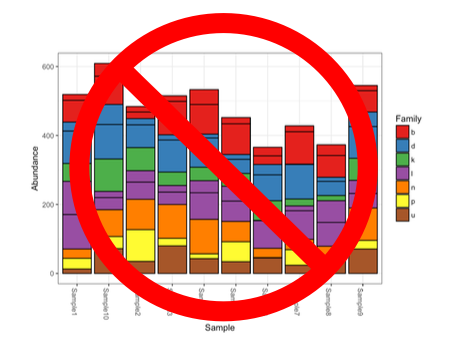
They gotta go. Specifically, I mean the stacked bar plot of raw uncorrected proportional abundances from metabarcoding data. Because amplification efficiencies impact the number of reads observed, you don’t know if one species is more abundant than another species because it is actually more abundant or because it just happens to amplify better than the other taxa in that sample.
Just don’t do it.
That being said, if you correct for amplification bias then by all means, use the stacked bar plots. Just know that you have to correct for amplification efficiencies beforehand. Otherwise, you are misrepresenting your data…
So now that I have rambled through our partial solutions and future directions, I have probably left you moderately to deeply unsatisfied and ready to throw in the towel for eDNA metabarcoding.
So to end on a high note, I leave you with one more blog post …
Unifying Theory of eDNA – Reconstructing Abundances from Metabarcoding Data
A bold statement. Certainly, whatever I am about to write in this next blog post will be wrong. All models are wrong, but some are useful. Hopefully this is at least helpful framework for how I have been thinking about going from observed sequence reads to reconstructing absolute abundances of species from eDNA.
The above mechanistic framework that we have proposed goes from DNA in your extraction through to sequencing.
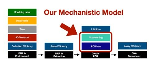
However, we know that there are a TON of factors that influence how much DNA ends up in the DNA extraction for metabarcoding, especially from an eDNA sample. So the next frontier is linking our framework to the great work already being done trying to model all of these various upstream components that are influencing how much DNA ends up in our extractions to the DNA in our bottles of water collected in the field to the number/abundance of organisms in the wild.
Here is a non-exhaustive list of things that we know influence the amount of DNA you get in a bottle of water:
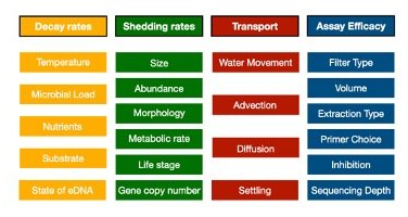
So in order to get to the abundances of actual organisms from observed sequence reads, we are going to need to parameterize each of these in the lab and in the field to know their relative contributions. And each of these little boxes themselves may interact with each other or have very important sub-boxes (e.g. morphology can incorporate both allometric scaling effects as well as dermal physiology). Parameterizing these values will be key to moving beyond the DNA extraction into the abundances of organisms in the wild. And thus, a grand unifying theory of eDNA would account for all of these various factors to explain observed sequence read distributions and link them to underlying organismal abundance in the wild.
I present a first, awkward step towards a unified theory of eDNA:
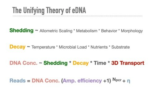
Now this might at first seem absolutely horrifying. There are easily +200 parameters we can all think of that might matter. There’s no way we will be able to measure of all these in the field. Every site is different. Every day of sampling has different conditions. It’s just not gonna happen.
But I don’t worry, I have hope. What is critically important to remember is that this they “might” matter.
We also get lots of eDNA results, particularly from the qPCR world that find the following:

So clearly, we must be doing something right. This is the kind of nice fit and limited variation that let’s fisheries ecologists sleep at night. Lord knows we wish standing stock biomass predicted recruitment this well. Would make everyone’s lives a lot easier.
Another thing that gives me hope from our metabarcoding work is that all of the other parameters in the equation pale in comparison to the amplification efficiency term. We are talking about something on the order of 235 (~34 billion). We are talking about a very very very large number. Correcting for this bias is going to account for a LOT of the observed variation. Gene copy number is important, particularly for protists and microbes with their Russian doll inception of endosymbionts, but still, that’s a factor of 3 or 4 tops in most cases. And probably a lot less of an issue for fish/vertebrates, although who knows how mtDNA concentrations vary across species and eDNA sources…
We also know that we can get fine-scale variation in eDNA signatures, particularly in marine environments where spatial variation is on the order of 10s of meters, temporal variation on the order of hours, and depth variation on the order of meters. These all suggest shedding rates are high, decay rates are fast, and transport is reasonable (meters not kilometers). This also strongly suggests that the integrated eDNA signature obtained from the environment is biased towards who is here and who is now. There is no doubt DNA can be transported pretty far and that it will be system dependent. Do your pilot studies, quantify those parameters, and inform your sampling design.
However, At the end of the day eDNA is clearly working and the literature is full of great examples. With all the great progress in the field, we can start putting down numbers to play out a lot of these scenarios on the back of a bar napkin and have a lot fewer “what ifs” with which parameters matter for eDNA and going from observed sequence reads to absolute abundance estimates.
Is eDNA going to get us accurate abundance estimates every time? Absolutely not. But neither do beach seines. We can’t let perfect be the enemy of the good. We can still operationalize eDNA for ecosystem assessments and biomonitoring if we don’t have every facet of variation nailed down.
This unifying framework provides us with a road map for how to link sources of variability in the lab to sources of variability in the field. Accounting for all these sources of variability will be critical for obtaining accurate quantitative abundance from eDNA metabarcoding data. And figuring out which estimates matter most will help us narrow down on the important components to measure in the field.
I whole heartedly agree, we can’t tackle a problem with this many parameters alone. Fortunately, folks are using eDNA all over the world and already doing all of the great hard work to parameterize these important pieces of variation. Brick by brick, parameter by parameter, we will build out this unifying theory of eDNA. I’m looking forward to how far we will be 10 years from now when we know the answers to nearly all of these components and the 10 more variables we should have been thinking about, but clearly didn’t in 2022.
Happy eDNA’ing and can’t wait to build out this unifying theory together with you all 🙂